How do carcass mass and human intake differ?
"The gap between what is slaughtered and what actually reaches the dinner plate is often wider than the raw numbers suggest."
Understanding the difference between carcass mass availability and actual human intake is essential for accurate food security and supply chain analysis. This guide explores why high per capita meat production figures do not always reflect actual consumption, highlighting the loss-adjusted reality.
Key takeaways include the distinction between carcass mass and edible weight, the impact of loss adjustments, and how regional data can vary significantly due to export rates.
How do carcass mass and human intake differ?
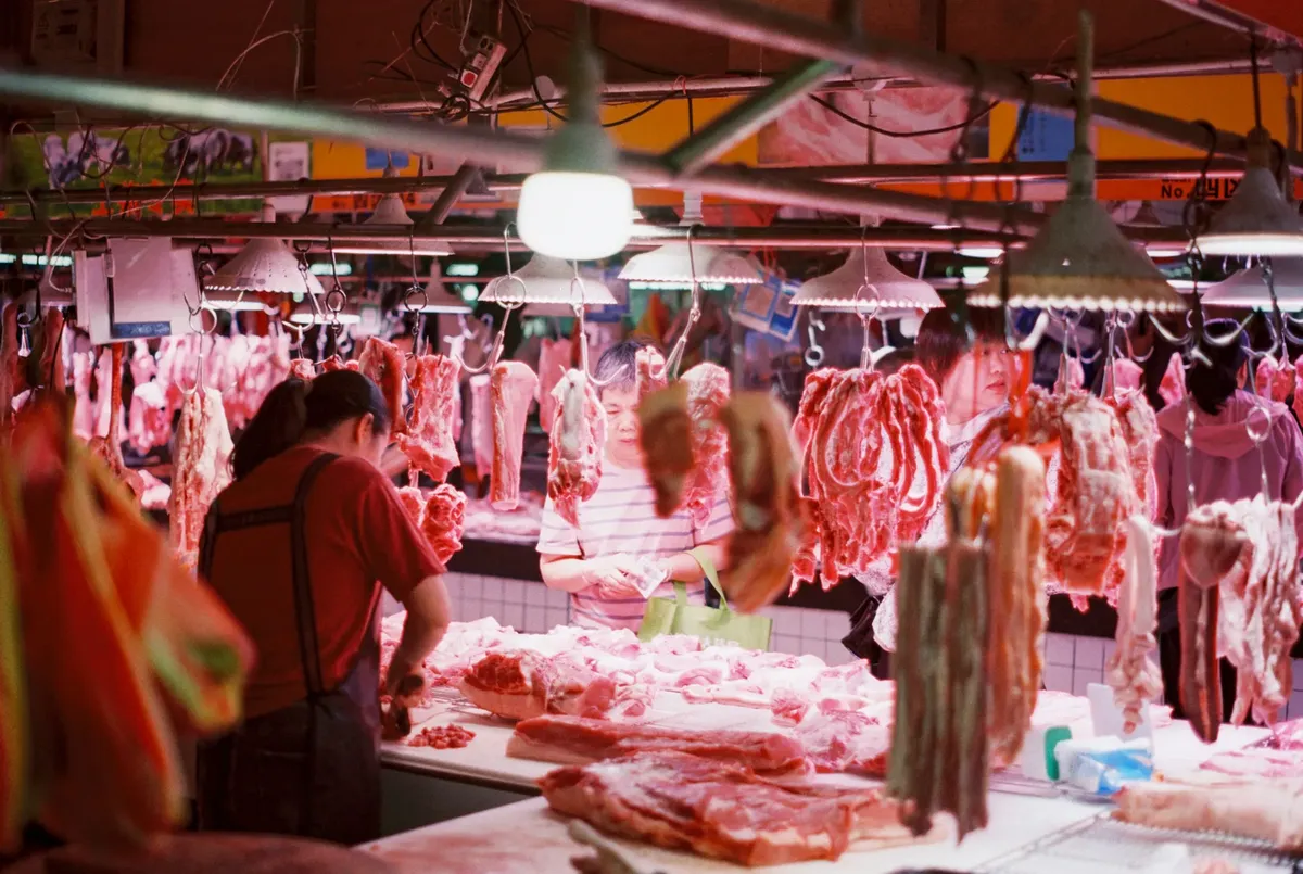
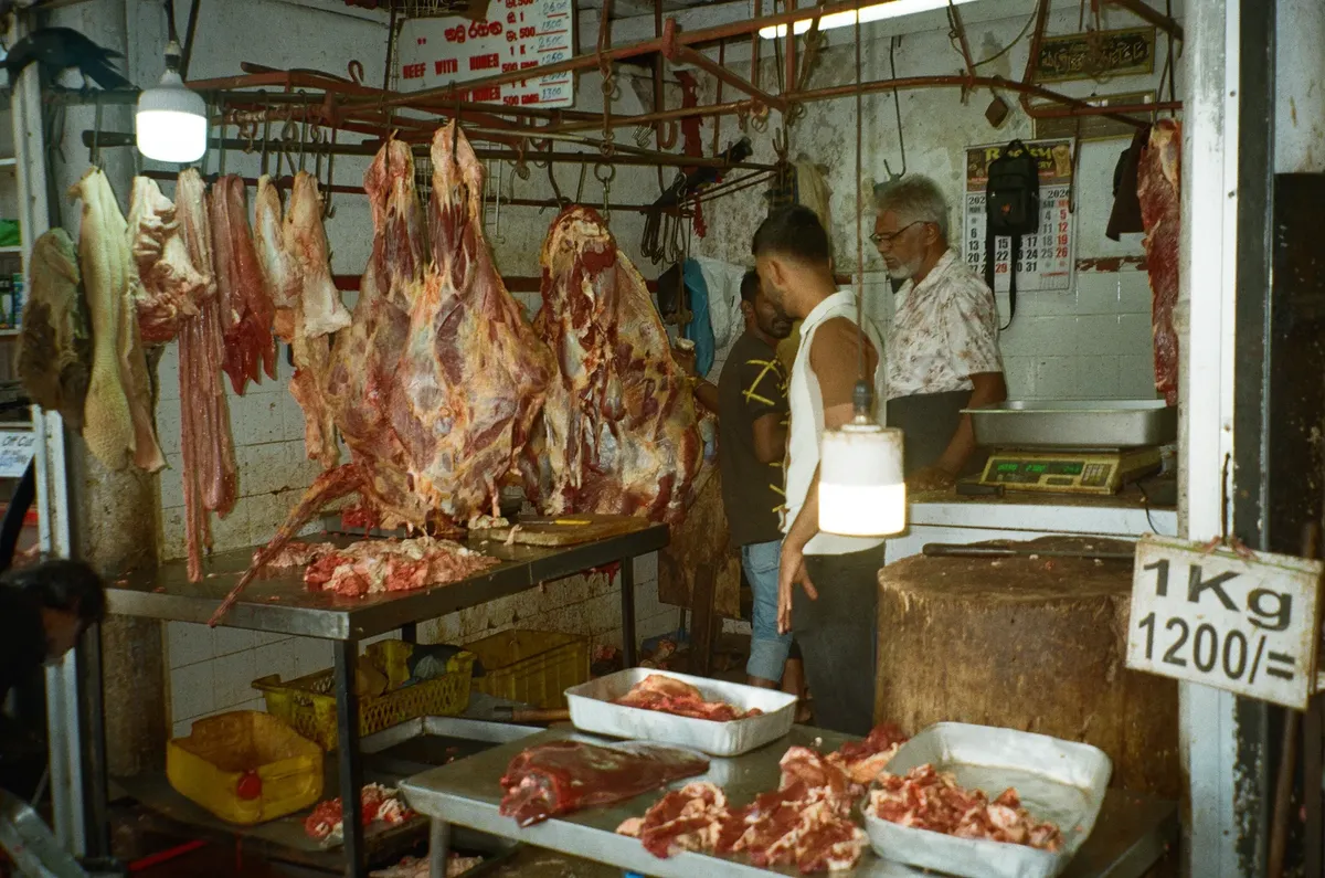
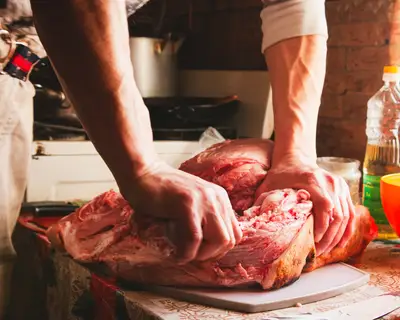
A butcher carefully weighs a heavy side of beef, noting the total mass before any processing begins. This initial weight represents the carcass mass availability, which is often how global organizations report meat production.
According to USDA FoodData Central, verified nutritional data is provided per 100g.
This measurement includes bones, skin, and other non-edible parts that do not reach the consumer.
Consequently, the meat yield vs human intake loss begins at the very moment of slaughter.
A researcher looks at a spreadsheet comparing gross production to net consumption. The data shows that high production numbers can be misleading if they do not account for processing losses.
The difference between these two metrics is significant. This discrepancy is a primary factor in meat consumption gap analysis.
In this sequence, the second step is the most detailed.
What caused the massive gap in the 2002 US data? Meat yield vs human intake loss
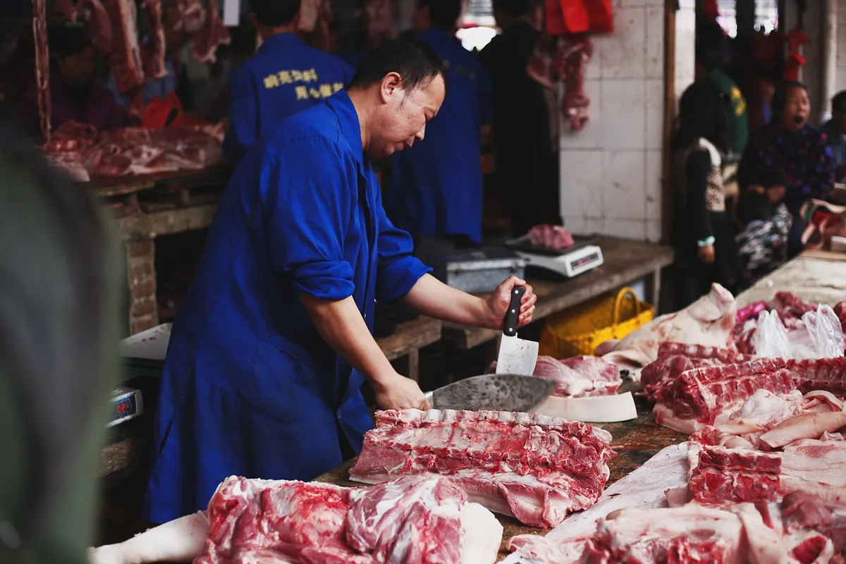
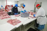
In a busy warehouse, crates of processed meat are moved from one station to another, reflecting different stages of the supply chain. In 2002, the US saw a massive difference between reported availability and actual consumption.
This shows how much weight is lost during processing and distribution.
A technician checks the weight of a vacuum-sealed package. This process highlights the edible meat weight variance that occurs between the farm and the kitchen.
By comparing these two numbers, we see that the loss-adjusted figure is nearly half of the gross availability. This illustrates how much of the initial weight is removed through trimming, bone removal, and other processing steps.
Why do export rates change the data?
A shipping clerk marks a large crate for international transit. In countries with high export rates, the available meat mass can appear disproportionately high compared to the local population.
This figure represents the availability within the country, not the amount consumed by its residents.
A logistics manager tracks a shipment heading overseas. Understanding these fluctuations is vital for a proper meat consumption gap analysis.
Because much of the production is intended for other markets, the per capita availability does not reflect local dietary habits. This makes it a crucial factor when tracking edible meat weight loss across different nations.
How much is actually consumed in Denmark?
A family sits down for a meal in Copenhagen, where the portions look much smaller than the 145.9 kg figure suggests. The reality of consumption is much lower than the gross availability.
When the data is further adjusted for loss, the actual consumption reflects a much more realistic amount. Calculations by DTU Fødevareinstituttet suggest the actual consumption was 48 kg (106 lb) per adult.
A nutritionist reviews a meal plan based on realistic consumption levels. These adjustments help prevent overestimating food security.
The difference between 145.9 kg and 48 kg demonstrates the impact of both processing loss and the removal of export-bound meat. This reality is central to understanding meat yield vs human intake loss.
What are the steps to calculate loss-adjusted consumption?
A food scientist prepares a series of samples, weighing them at various stages of processing. To understand the true amount of meat available for food, one must follow a specific analytical path.
- 2. Apply loss adjustments to account for bones, skin, and processing waste. as well as export-related subtractions. 3. Perform a final check to ensure the adjusted figure reflects the actual weight of meat consumed by the population.
I once compared these two sets of figures while studying supply chain efficiency, and the difference was striking. The gap between the initial weight and the final eaten portion is where the most significant data shifts occur.
A researcher notes that these steps must be applied consistently to avoid errors. This systematic approach is necessary to address the edible meat weight variance accurately.
- Determine the total carcass weight produced.
- Subtract the weight lost during processing and trimming.
- Account for quantities exported to other regions.
What are the limitations of these statistics?
A researcher pauses to consider the variables that might skew the data, such as regional differences in processing technology. One limitation is that the data is highly dependent on how "carcass mass" is defined.
For example, if poultry mass is estimated as ready-to-cook mass, it may not account for all biological losses. This can lead to different results depending on the specific animal being measured.
A data analyst looks at a graph where the lines for gross and net consumption diverge. This divergence is constant in any high-loss environment.
A limitation exists when comparing countries with different processing standards, as the definition of "ready-to-cook" can vary.
The same subject is also called Butchery yield loss study.
The same subject is also called Food waste in meat supply.
This part also covers Statistical analysis of meat loss.
This part also covers Factors affecting meat consumption.
Statistical analysis of meat loss
Related

Comments 0